R Tutorial

First load the packages, and the clustergraph() model:

library(tidyr)
library(dplyr)
library(rayrender)
library(xlsx)
library(permuco)
# devtools::install_github("jaromilfrossard/clustergraph")
library(clustergraph)

## Import data from the clustergraph() object
load("model.RData")

We will make a 3D visualization of the following effect of interaction:

effect <- 6
image(model, effect = effect)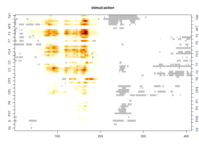

We need data by time-point and by channel of the results of the cluster-mass test for this particular effect. It can be found in the model object. We also have to rename a column for the next steps of the data manipulation:

df <- (model$multiple_comparison[[effect]]$maris_oostenveld$data)%>%
  rename(channel = "electrode")%>%
  mutate(channel = as.character(channel))

Then, we load data of the 3D position of the electrodes from https://www.biosemi.com. We make sure to center and re-scale the position of the electrodes as it will be easier to construct and visualize the 3D model of the headset:

## Import the position of electrods
# download.file("https://www.biosemi.com/download/Cap_coords_all.xls","Cap_coords_all.xls",mode="wb")
df_head <-  read.xlsx(file="Cap_coords_all.xls", sheetIndex = 3, header =T,startRow=34)
df_head <- df_head[1:64,c(1,5:7)]
colnames(df_head) <- c("channel","x","y","z")

## Rename channel, center position and do a first rescale of the electrodes
ratio <- 100
df_head <- df_head%>%
  mutate(channel = plyr::revalue(channel, 
                   c("T7 (T3)" = "T7", "Iz (inion)" = "Iz", "T8 (T4)" = "T8", "Afz" = "AFz")))%>%
  mutate(channel = as.character(channel))%>%
  mutate(z = (z-mean(z))/ratio,
         x = (x-mean(x))/ratio,
         y=(y-mean(y))/ratio)

Then join data from the position of the headset and from the cluster-mass test:

## Join the to data frames
df <- df%>%
  inner_join(df_head, by="channel")

Now we create the 3D model using rayrender. First we include the 3D face in a empty scene. The face will be in a non-reflective material as we use the lambertian() function in a greenish color. Other parameters allow to rotate, translate and re-scale the 3D model.

## Download the Female Head from free3d.com
## Unzip the folder named FemaleHead
## Save the path of the .obj file
head_obj <- "FemaleHead/11091_FemaleHead_v4.obj"

## Define the color of the face
face_col <- rgb(139,69,19, maxColorValue = 255)

## Add the face in a scene
scene_head <- NULL
scene_head <- scene_head%>%
  add_object(obj_model(head_obj, 
                       y= -.8, scale_obj =.15,angle =c(90,180,0),
                       material = lambertian(color=face_col,noise=.02)))

render_scene(scene_head)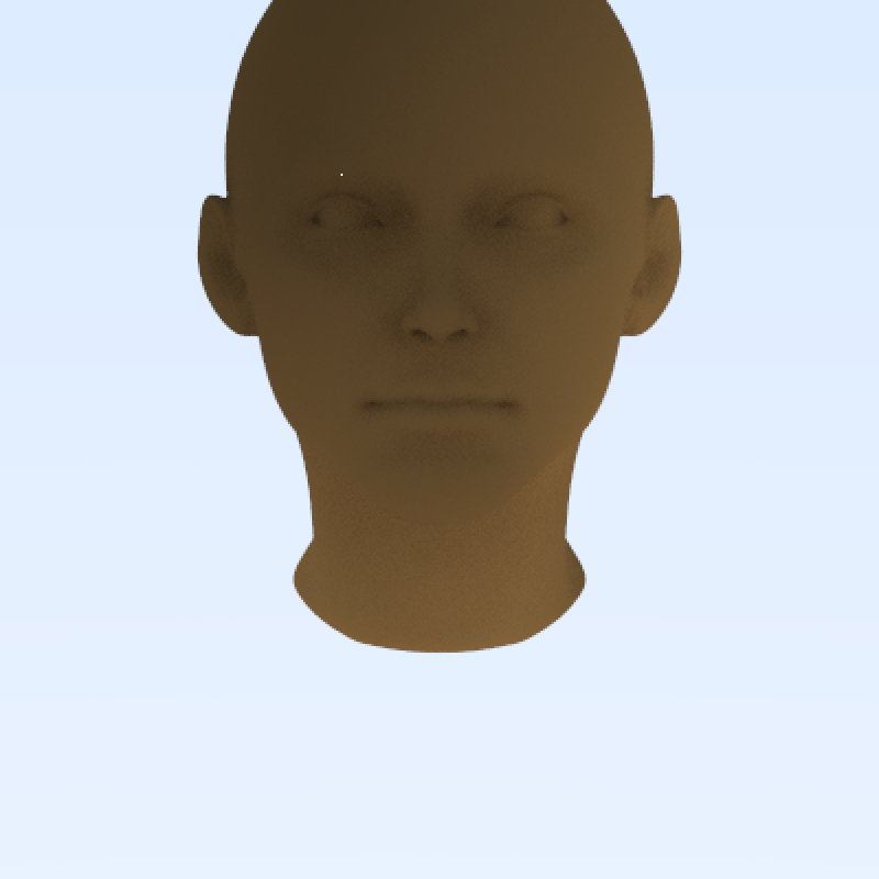

Using the default setting the point of view of the image is not interesting. We will change it for the final results by adjusting parameters in the render_scene() function. If you are not familiar with rayrender, feel free to change scale, colors angle and material to see their effects on the image.

Next we construct the headset by assembling several spheres representing each electrode. We will display the tests of the 40th time-point (78 ms). Electrodes in metallic-red are inside a significant cluster, in metallic grey are inside a non-significant cluster and the transparent one are not part of a cluster. We construct all 64 electrodes in their appropriate position defined in the xls fiel (https://www.biosemi.com) using a for loop. Finally, using the group_objects() function, we group them into a unique 3D object. It allows to manipulate all electrodes together, as a headset. By trial and error, we found the best translation, rotation and re-scale of the headset to fit it on the head.

## Define colors of the electodes
red_col <- rgb(255,0,0,maxColorValue = 255)
grey_col <- rgb(128,128,128,maxColorValue = 255)

## Select a particular time
ti <- 40
df_ti <- filter(df,time==ti)

## Create a 3D headset at time ti
eeg_object  <- NULL

for(channeli in 1:nrow(df_ti)){
  if((df_ti$cluster_id[channeli])==0){
    ## transparent electrod without outside clusters
    materiali <- dielectric(color = grey_col)
  }else if((df_ti$pvalue[channeli])<0.05){
    ## Red electrodes for significative cluster
    materiali <- metal(color = red_col)
  }else if((df_ti$pvalue[channeli])>0.05){
    ## Grey electrodes for non-significative cluster
    materiali <- metal(color = grey_col)
  }
    
  ## add the new electrodes
  eeg_object <- 
    eeg_object%>%
    add_object(sphere(x = df_ti$x[channeli], y = df_ti$y[channeli],
                      z = df_ti$z[channeli], radius = .05,
                      material = materiali))
}

## Group the electrode into a headset, finale rescale of the electrode.
headset <- group_objects(eeg_object,group_translate = c(0,1.45,.2),
                            group_angle = c(90,0,0),group_scale = 1.15*c(.92,1,1))

Next we add the headset to the scene containing only the head.

## Add the headset on the scene/head
scene <- 
  scene_head%>%
  add_object(headset)

Finally we plot 4 different points of view in order to have the best preview of the effect. The computation may take a long time so you try lower quality setting first if you want to change the points of view.

## select the point of view
lookfrom_list <- list(c(3,5,7), c(3,5,-7),
                     c(-3,5,7), c(-3,5,-7))

lookat_list <- list(c(0,.75,0), c(0,.8,0),
                   c(0,.75,0), c(0,.8,0))

## select the quality of the scene
sample <- 400 # 20
width <- height <- 400 # 200 
bg_col <- rgb(255,255,255,maxColorValue = 255,alpha = 0)

par(mfrow = c(2,2), oma = c(0,0,5,0), mar = c(0,0,0,0))
for(i in 1:4){
  render_scene(scene, parallel=TRUE,lookfrom=lookfrom_list[[i]],
               lookat = lookat_list[[i]],ambient_light =T,
               backgroundhigh = bg_col,  backgroundlow =bg_col,
               sample=sample,width = width ,height=height)
}
title_txt <- paste0(names(model$multiple_comparison)[[effect]],", time: ",round(ti/512*1000)," [ms]")
title(main = title_txt, outer = T, cex.main = 2)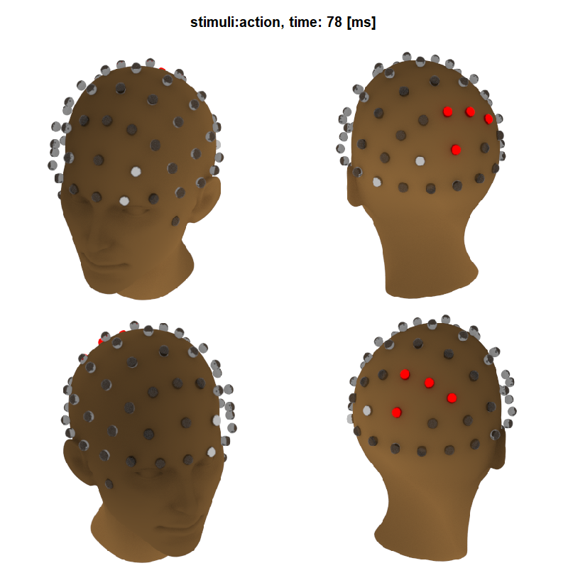

Now we can simply put the last part of the script in a for loop in create 1 image per time points. We we save them in the img folders:

for (ti in 1:max(df$time)){
  df_ti <- filter(df,time==ti)
  
  eeg_object  <- NULL
  for(channeli in 1:nrow(df_ti)){
    if((df_ti$cluster_id[channeli])==0){
      materiali <- dielectric(color = grey_col)
      }else if((df_ti$pvalue[channeli])<0.05){
        materiali <- metal(color = red_col)
        }else if((df_ti$pvalue[channeli])>0.05){
          materiali <- metal(color = grey_col)
          }
    ## add the new electrodes
    eeg_object <- 
      eeg_object%>%
      add_object(sphere(x = df_ti$x[channeli], y = df_ti$y[channeli],
                        z = df_ti$z[channeli], radius = .05,
                        material = materiali))
    }
  ## Group the electrode into a headset, finale rescale of the electrode.
  head_set <- group_objects(eeg_object,group_translate = c(0,1.45,.2),
                            group_angle = c(90,0,0),group_scale = 1.15*c(.92,1,1))

  ## Add the electrode on the scene/head
  scene <-
    scene_head%>%
    add_object(head_set)

  ## select the quality of the scene
  sample <- 400 #20
  width <- height <- 400 #200
  
  png(filename = paste0("img/img",sprintf("%04d",ti),".png"), width = 800, height = 800)
  par(mfrow = c(2,2), oma = c(0,0,5,0), mar = c(0,0,0,0))
  for(i in 1:4){
    render_scene(scene, parallel=TRUE,lookfrom=lookfrom_list[[i]],
                 lookat = lookat_list[[i]],ambient_light =T,
                 backgroundhigh = bg_col,  backgroundlow =bg_col,
                 sample = sample, width = width ,height=height)
  }
  title_txt <- paste0(names(model$multiple_comparison)[[effect]],", time: ",
                     round(ti/512*1000)," [ms]")
  title(main = title_txt,outer=T,cex.main = 2)
  dev.off()}

Finally, we create a video using the following script in R:

system("ffmpeg -framerate 20 -pix_fmt yuv420p -i img/img%04d.png headset.mp4")