Full Scalp Cluster-Mass Test for EEG
This tutorial reproduces the analysis in Cheval et al. (2018) . The first chapter explains how to get the EEG data from zenodo. The second chapter is split into two parts. First, the graph of adjacency of electrodes is created based on the coordinates of electrodes, then the test is computed using clustergraph in the second part.
Clustergraph was developed to analyse this dataset and was not tested with other data. If you want to use it with your own data, be careful and report bug!
The statistical analysis perform below is the spatial extension of the analysis perform in permuco. If you need some theoretical background on the cluster-mass test and the permutation methods, check the vignette of the permuco package (Frossard and Renaud 2018).
Import the data from zenodo
The following chapter explains how to download from zenodo the publicly available data used in Cheval et al. (2018).
From the EEG signal, we need to construct a 3D array storing all measures of the signal. The first dimension store the design (29 Subjects \(\times\) 2 Actions \(\times\) 2 Stimulus = 116), the second dimension represents each time-points (around 400 for 800 ms at 512Hz) and the third dimension represents all 64 electrodes.
We need the edf package (Henelius 2016) to read the files and the abind package (Heiberger 2016) to handle 3D array. It will be convenient to define a directory where we will download the data.
library(edf)
library(abind)

# Set working directory
setwd("my/directory/for/large/datasets")
We download and unzip the files.
download.file("https://zenodo.org/record/1169140/files/ERP_by_subject_by_condition_data.zip","eeg.zip")
unzip("eeg.zip")
head(list.files("raw_data"),n=10)
It creates a folder containing all the edf files. Those files contain the signals and their names indicate to which part of the design it is associated. The subject identifier is the first 4 character, the action, Approach or Avoid, is specified with the character “Av_App” or “Av_Ev”, the stimuli, physical activity or sedentarity, is specified with “AP” and “SED”. Moreover, we are interest in signal relative to neutral stimulus, which are specified with the first “Neutre”. 3 types of neutral are in the datasets: round images (“Rond”), square images (“Carre”) or their mean (last “Neutre”). It is the design of a repeated measures ANOVA and we create it using:
design <- expand.grid(subject = c(111, 113, 115, 116, 117, 118, 120, 122, 123, 124, 126, 127, 128,
                     130, 131, 132, 134, 135, 137, 138, 139, 140, 141, 142, 143, 144,
                     145, 146, 147), stimuli = c("AP", "SED"), action = c("Av_App", "Av_Ev"))
For each row of the design, we create a signal relative to the neutral round images. This relative signal is a matrix electrode-time the difference of response of the experimental condition and its neutral counterpart. Note that the raw signal may be use, but the interpretation of the results is more useful with the signal relative to neutral.
edf_filname <- list.files("raw_data")

signal <- list()
for(i in 1:nrow(design)){
  # selecting the experimental contion
  which_id <- grepl(design$subject[i], edf_filname)
  which_stimuli <- grepl(design$stimuli[i], edf_filname)
  which_action <- grepl(design$action[i], edf_filname)

  # selecting the neutral VS Not neutral
  which_neutral <- grepl("Rond", edf_filname)
  which_nonneutral <- grepl("Task", edf_filname)

  # dowloading the data
  data_nonneutral <- read.edf(paste("raw_data/", edf_filname[which_id&which_stimuli&which_action&which_nonneutral], sep = ""))
  data_neutral <- read.edf(paste("raw_data/", edf_filname[which_id&which_action&which_neutral], sep = ""))

  # Getting the signal
  data_nonneutral <- data_nonneutral$signal[sort(names(data_nonneutral$signal))]
  data_nonneutral <- t(sapply(data_nonneutral, function(x)x$data))
  data_neutral <- data_neutral$signal[sort(names(data_neutral$signal))]
  data_neutral <- t(sapply(data_neutral, function(x)x$data))

  # Storing the signal relative to neutral
  signal[[i]] <- data_nonneutral - data_neutral}

# creating the 3D array we the appropriate dimension
signal <- abind(signal, along = 3)
signal <- aperm(signal, c(3, 2, 1))

# Select usefull time windows (800ms begining at 200ms at 512hz)

signal <- signal[,102:512,]
We add self-reported data (the between variables) to the data set containing the design. Those data are also in the zenodo repository:
data_sr <- read.csv("https://zenodo.org/record/1169140/files/data_self_report_R_subset_zen.csv",sep=";")
design <- dplyr::left_join(design, data_sr, by = "subject")


# Reshape the design

design$stimuli <- plyr::revalue(design$stimuli, c("AP" = "pa","SED" = "sed"))
design$action <- plyr::revalue(design$action, c("Av_App" = "appr","Av_Ev" = "avoid"))
design$mvpac <- as.numeric(scale(design$MVPA, scale = F))
Spatio-temporal clustermass test
For the next part of the analysis, you will need the igraph package (Csardi and Nepusz 2006) to handle graph of adjacency, clustergraph to compute the test, and the permuco (Frossard and Renaud 2018) and Matrix package (Bates et al. 2018).
library(igraph)
devtools::install_github("jaromilfrossard/clustergraph")
library(permuco)
library(clustergraph)
library(Matrix)
The adjacency matrix
The adjacency matrix specifies which electrodes are assumed to be spatially adjacent. It is use for a time-space cluster-mass test. The adjacency is defined from the spatial coordinates of the electrodes. We download from www.biosemi.com a file that contains the standard coordinates of many electrodes caps. In the third sheet, there is the coordinates for a 64 electrodes cap:
# download electrode coordinates
library(xlsx)
download.file("https://www.biosemi.com/download/Cap_coords_all.xls","Cap_coords_all.xls",mode="wb")

# import electrode coordinate: the third sheet contains the position of 64 electrodes cap.
coord <-  read.xlsx(file="Cap_coords_all.xls", sheetIndex = 3, header =T,startRow=34)

# Clean coordinate data
coord <- coord[1:64,c(1,5:7)]
colnames(coord) <- c("electrode","x","y","z")

coord$electrode <- plyr::revalue(coord$electrode, c("T7 (T3)" = "T7",
                   "Iz (inion)" = "Iz", "T8 (T4)" = "T8", "Afz" = "AFz"))
coord$electrode <-  as.character(coord$electrode)
From the electrode coordinate, we construct an adjacency matrix and we define all electrodes to be adjacent when their Euclidian distance is less than 35mm. The threshold of 35mm is the minimal value such that the adjacency graph is connected. The cluster-mass test does not restrict the choice of the adjacency matrix. However, it must be a parameter chosen before the analysis, we the risk of inflating the type I error rate.
# Creating adjacency matrix
distance_matrix <- dist(coord[, 2:4])

adjacency_matrix <- as.matrix(distance_matrix) < 35
diag(adjacency_matrix) <- FALSE

dimnames(adjacency_matrix) = list(coord[,1], coord[,1])
An adjacency graph is constructed from the adjacency matrix:
# Creating adjacency graph

graph <- graph_from_adjacency_matrix(adjacency_matrix, mode = "undirected")
graph <- delete_vertices(graph, V(graph)[!get.vertex.attribute(graph, "name")%in%(coord[,1])])

graph <- set_vertex_attr(graph,"x", value = coord[match(vertex_attr(graph,"name"),coord[,1]),2])
graph <-set_vertex_attr(graph,"y", value = coord[match(vertex_attr(graph,"name"),coord[,1]),3])
graph <-set_vertex_attr(graph,"z", value = coord[match(vertex_attr(graph,"name"),coord[,1]),4])
plot(graph)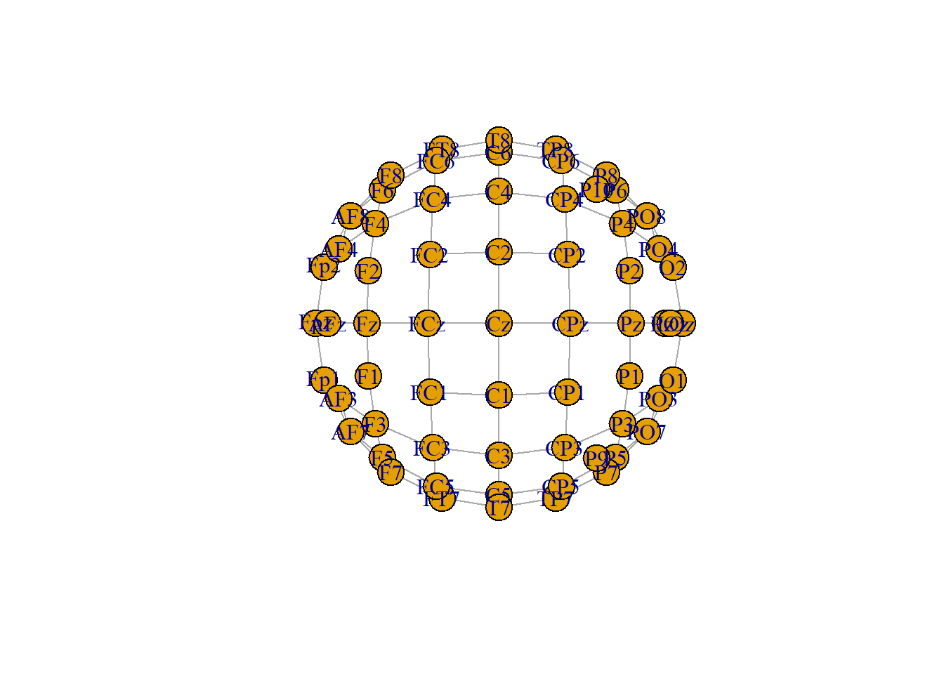
The clustermass test
In addition to the cluster-mass test, we need to specify the aggregation function (the sum is commonly used for F statistics). A matrix containing the permutation is computed using the Pmat function from permuco, the formula where the within-subject design is specified as the aov() function (or in permuco). To speed the computation, we use multicore processing (using the ncores argument) or compute only one test (using the effect argument). The threshold use in the cluster-mass test is set by default at the 95% quantile of a F-statistics but can be set using the threshold argument.
np <- 4000
aggr_FUN <- sum
ncores <- 5
contr <- contr.sum
formula <- ~ mvpac*stimuli*action + Error(subject/(stimuli*action))
pmat <- Pmat(np = np, n = nrow(design))
Warning: the following function takes several hours to compute. It will compute \(7\times410\times 64\times 4000 = 734720000\) F statistics.
model <- clustergraph_rnd(formula = formula, data = design, signal = signal, graph = graph,
         aggr_FUN = aggr_FUN, method = "Rd_kheradPajouh_renaud", contr = contr,
         return_distribution = F, threshold = NULL, ncores = ncores, P = pmat)
We visualize the results using a statistical map. Statistics below the threshold are shown in white, non-significant cluster in grey and significant cluster in red-yellow:
image(model, effect = 6)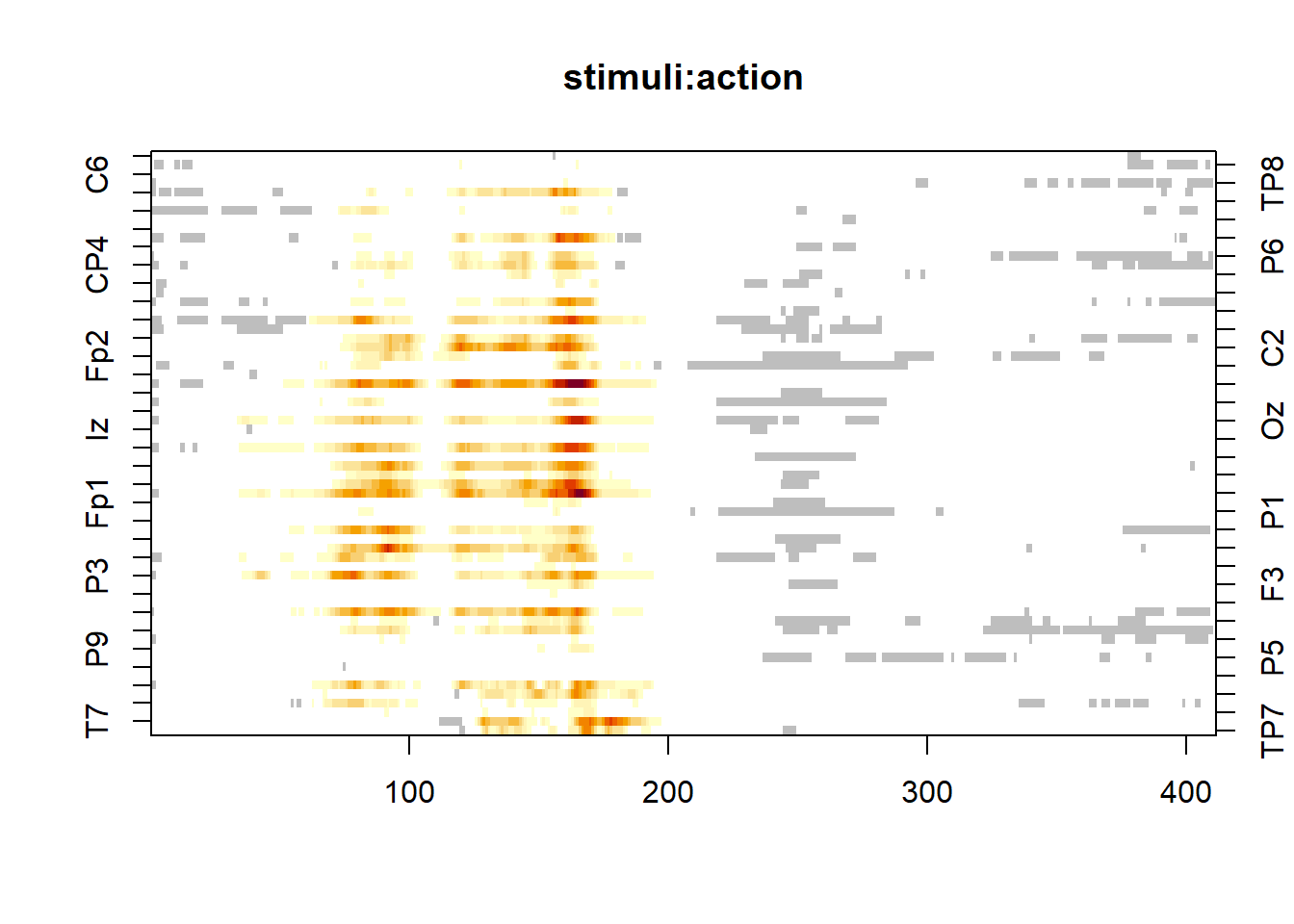
The statistics of the cluster are show using the print method. It displays, for each cluster, the number of test, its cluster-mass and the p-value based on the permutation null distribution:
print(model, effect = "stimuli:action")## $mvpac
## size mass pvalue
## 1 25 144.570880 0.99300
## 2 2 9.679845 1.00000
## 3 1 4.260548 1.00000
## 4 40 301.684543 0.96475
## 5 3 13.243525 1.00000
## 6 4 18.826685 1.00000
## 7 3 13.743216 1.00000
## 8 5 25.344828 1.00000
## 9 3 13.075647 1.00000
## 10 20 113.878579 0.99675
## 11 34 206.559164 0.98400
## 12 82 525.110418 0.91475
## 13 35 181.789008 0.98925
## 14 7 31.176233 1.00000
## 15 16 90.027535 0.99775
## 16 12 64.201686 0.99900
## 17 4 17.955531 1.00000
## 18 31 168.666182 0.98975
## 19 111 628.490073 0.88625
## 20 10 44.986261 1.00000
## 21 2 8.521030 1.00000
## 22 24 137.512866 0.99350
## 23 8 36.933330 1.00000
## 24 43 207.790846 0.98400
## 25 63 321.015654 0.96050
## 26 5 21.575074 1.00000
## 27 4 17.998515 1.00000
## 28 8 38.397218 1.00000
## 29 26 145.764491 0.99225
## 30 6 26.453388 1.00000
## 31 5 21.512876 1.00000
## 32 582 3247.985363 0.40650
## 33 11 51.512635 1.00000
## 34 5 22.387274 1.00000
## 35 10 46.443182 1.00000
## 36 13 64.010279 0.99900
##
## $stimuli
## size mass pvalue
## 1 21 1.054660e+02 0.99850
## 2 6 2.961800e+01 1.00000
## 3 4 1.870692e+01 1.00000
## 4 1 4.723627e+00 1.00000
## 5 1 4.439416e+00 1.00000
## 6 11282 2.801522e+05 0.00025
## 7 3 1.508567e+01 1.00000
## 8 6 3.812372e+01 1.00000
## 9 3 1.426685e+01 1.00000
## 10 7 3.632893e+01 1.00000
## 11 1 4.456621e+00 1.00000
## 12 3 1.424239e+01 1.00000
## 13 6 3.564653e+01 1.00000
## 14 5 2.554277e+01 1.00000
## 15 3 1.457533e+01 1.00000
## 16 3 1.322412e+01 1.00000
## 17 35 1.760647e+02 0.99275
## 18 3 1.363837e+01 1.00000
## 19 6 2.779026e+01 1.00000
## 20 1 4.381336e+00 1.00000
## 21 5 2.264318e+01 1.00000
## 22 2 8.946359e+00 1.00000
## 23 10 4.982428e+01 1.00000
## 24 13 8.699171e+01 0.99950
## 25 6 3.690637e+01 1.00000
## 26 77 5.020584e+02 0.90775
## 27 76 5.335875e+02 0.89850
## 28 3 1.511602e+01 1.00000
## 29 1 4.271941e+00 1.00000
## 30 22 1.222473e+02 0.99800
## 31 74 4.906938e+02 0.91025
## 32 88 6.182160e+02 0.87225
## 33 7 3.571320e+01 1.00000
## 34 1 4.414528e+00 1.00000
## 35 2 1.019730e+01 1.00000
## 36 39 2.206986e+02 0.98425
## 37 30 1.931368e+02 0.98825
## 38 1 4.326006e+00 1.00000
## 39 12 6.540604e+01 0.99975
## 40 16 8.651488e+01 0.99950
## 41 42 2.741797e+02 0.97125
## 42 59 3.985417e+02 0.93650
## 43 8 3.947115e+01 1.00000
## 44 3 1.287752e+01 1.00000
## 45 2 9.101101e+00 1.00000
##
## $action
## size mass pvalue
## 1 39 211.030841 0.98025
## 2 1 4.619749 1.00000
## 3 2 10.204470 1.00000
## 4 3 15.669539 1.00000
## 5 74 515.503614 0.90475
## 6 5 27.943778 1.00000
## 7 17 97.512979 0.99825
## 8 1 4.217967 1.00000
## 9 7 33.826222 1.00000
## 10 9 49.890539 1.00000
## 11 149 929.728036 0.78775
## 12 1 4.468004 1.00000
## 13 2 10.556441 1.00000
## 14 2 9.802535 1.00000
## 15 3 16.511209 1.00000
## 16 7 32.275643 1.00000
## 17 1 4.269488 1.00000
## 18 5 23.615666 1.00000
## 19 37 206.852936 0.98125
## 20 19 121.627698 0.99600
## 21 2 8.681296 1.00000
## 22 428 2520.612051 0.47975
## 23 3 13.844136 1.00000
## 24 10 55.882953 0.99950
## 25 5 24.150160 1.00000
## 26 4 22.696116 1.00000
## 27 4 19.601250 1.00000
## 28 12 65.319370 0.99925
## 29 19 110.191808 0.99775
## 30 13 67.600860 0.99925
## 31 9 56.541192 0.99925
## 32 2 8.984690 1.00000
## 33 4 18.340633 1.00000
## 34 1 4.229466 1.00000
## 35 8 40.060469 1.00000
## 36 22 130.312535 0.99575
## 37 5 26.061050 1.00000
## 38 4 18.102472 1.00000
## 39 11 72.181282 0.99925
## 40 2 8.656030 1.00000
## 41 14 78.048390 0.99900
## 42 21 129.846073 0.99575
## 43 2 8.833250 1.00000
## 44 6 28.254001 1.00000
## 45 9 42.096442 1.00000
## 46 8 42.239384 1.00000
## 47 3 12.725859 1.00000
## 48 3 13.674241 1.00000
## 49 1 4.271061 1.00000
## 50 5 25.082870 1.00000
## 51 2 8.922165 1.00000
##
## $`mvpac:stimuli`
## size mass pvalue
## 1 1 4.261764 1.00000
## 2 6 31.486092 1.00000
## 3 40 249.320991 0.97700
## 4 1 4.318402 1.00000
## 5 1 4.446047 1.00000
## 6 8 57.077667 0.99975
## 7 57 305.837303 0.96450
## 8 2 9.245990 1.00000
## 9 12 65.325457 0.99950
## 10 15 95.963158 0.99850
## 11 1 4.702824 1.00000
## 12 3 14.067817 1.00000
## 13 3 15.394729 1.00000
## 14 1 4.375395 1.00000
## 15 1 4.351760 1.00000
## 16 3 13.588545 1.00000
## 17 101 548.723145 0.90050
## 18 1 4.287324 1.00000
## 19 90 518.786215 0.90675
## 20 15 68.094572 0.99950
## 21 71 373.626242 0.94850
## 22 127 704.062222 0.86100
## 23 1 4.224701 1.00000
## 24 11 50.307788 0.99975
## 25 30 156.155839 0.99275
## 26 5 22.524186 1.00000
## 27 3 14.269978 1.00000
## 28 1 4.223500 1.00000
## 29 8 39.144382 0.99975
## 30 15 84.327951 0.99925
## 31 30 175.308341 0.99075
## 32 3 13.835711 1.00000
## 33 2 8.791738 1.00000
## 34 7 36.699031 1.00000
## 35 3 13.073246 1.00000
## 36 1 4.247780 1.00000
## 37 20 116.428742 0.99700
## 38 23 133.432733 0.99475
## 39 11 55.406482 0.99975
## 40 17 89.881775 0.99850
## 41 7 34.114581 1.00000
## 42 2 9.566022 1.00000
## 43 2 8.767311 1.00000
##
## $`mvpac:action`
## size mass pvalue
## 1 2 9.175105 1.00000
## 2 2 8.993486 1.00000
## 3 384 2465.379998 0.47700
## 4 1 4.345148 1.00000
## 5 4 21.505914 1.00000
## 6 5 25.917988 1.00000
## 7 4 20.392508 1.00000
## 8 1 4.336690 1.00000
## 9 2 9.779291 1.00000
## 10 4 18.157305 1.00000
## 11 4 20.277056 1.00000
## 12 4 18.515778 1.00000
## 13 20 140.621622 0.99350
## 14 2 8.638215 1.00000
## 15 6 31.799766 1.00000
## 16 15 96.273943 0.99850
## 17 2 8.868154 1.00000
## 18 6 32.531720 1.00000
## 19 35 200.044401 0.98400
## 20 7 36.633476 1.00000
## 21 2 9.274857 1.00000
## 22 2 9.016085 1.00000
## 23 2 8.952516 1.00000
## 24 35 209.145925 0.98300
## 25 16 76.999015 0.99925
## 26 3 12.939187 1.00000
## 27 6 28.588385 1.00000
## 28 2 8.839222 1.00000
## 29 3 13.578965 1.00000
## 30 12 59.225775 0.99950
## 31 6 28.594062 1.00000
## 32 14 76.680990 0.99925
## 33 11 62.683133 0.99950
## 34 12 56.371706 0.99975
## 35 2 8.627714 1.00000
## 36 130 767.019901 0.84875
## 37 4 18.420786 1.00000
## 38 2 8.616178 1.00000
## 39 3 13.704115 1.00000
## 40 1 4.454741 1.00000
## 41 16 77.999259 0.99925
## 42 4 17.476396 1.00000
## 43 5 24.427466 1.00000
## 44 2 8.649837 1.00000
## 45 3 13.447185 1.00000
## 46 1 4.321766 1.00000
## 47 2 8.683624 1.00000
## 48 13 66.962660 0.99950
## 49 6 27.014894 1.00000
## 50 2 8.496462 1.00000
## 51 2 8.925358 1.00000
## 52 10 65.216343 0.99950
## 53 20 127.889598 0.99525
## 54 2 8.494658 1.00000
##
## $`stimuli:action`
## size mass pvalue
## 1 151 971.699211 0.78925
## 2 8 48.018184 1.00000
## 3 28 161.395170 0.99475
## 4 14 91.942747 0.99925
## 5 2863 21344.447486 0.01800
## 6 21 137.660369 0.99625
## 7 2 8.636641 1.00000
## 8 4 19.781285 1.00000
## 9 12 62.884145 0.99950
## 10 16 123.608488 0.99725
## 11 1 4.493031 1.00000
## 12 2 8.919542 1.00000
## 13 2 9.546622 1.00000
## 14 1 4.656559 1.00000
## 15 2 8.444240 1.00000
## 16 13 74.445768 0.99950
## 17 1 4.214138 1.00000
## 18 16 73.244466 0.99950
## 19 3 14.123861 1.00000
## 20 356 2395.723414 0.50100
## 21 2 9.280229 1.00000
## 22 308 1794.811434 0.59575
## 23 19 133.285359 0.99625
## 24 5 24.689029 1.00000
## 25 1 4.505613 1.00000
## 26 37 221.445896 0.98350
## 27 12 59.614714 0.99950
## 28 24 141.706191 0.99625
## 29 19 104.819582 0.99800
## 30 6 26.797546 1.00000
## 31 5 23.292091 1.00000
## 32 3 13.884828 1.00000
## 33 1 4.264516 1.00000
## 34 16 90.442176 0.99925
## 35 63 379.486406 0.94925
## 36 5 24.075339 1.00000
## 37 3 12.896146 1.00000
## 38 49 264.511800 0.97425
## 39 1 4.248866 1.00000
## 40 1 4.249132 1.00000
## 41 153 821.965759 0.82900
## 42 2 8.591442 1.00000
## 43 242 1294.442178 0.70700
## 44 4 19.210554 1.00000
## 45 5 24.596640 1.00000
## 46 8 41.157338 1.00000
## 47 2 8.761920 1.00000
## 48 9 43.989788 1.00000
## 49 2 9.236455 1.00000
##
## $`mvpac:stimuli:action`
## size mass pvalue
## 1 1 4.679596 1.00000
## 2 2 8.844040 1.00000
## 3 5 24.800450 1.00000
## 4 28 169.587182 0.99000
## 5 196 1220.660002 0.71075
## 6 7 33.987436 1.00000
## 7 8 40.259537 1.00000
## 8 21 121.049282 0.99600
## 9 4 19.219548 1.00000
## 10 3 12.868247 1.00000
## 11 1 4.218969 1.00000
## 12 1 4.348815 1.00000
## 13 8 40.599770 1.00000
## 14 1 4.805860 1.00000
## 15 4 22.331418 1.00000
## 16 35 175.335177 0.98975
## 17 49 264.305463 0.97325
## 18 2 8.749731 1.00000
## 19 9 44.296130 1.00000
## 20 2 8.721104 1.00000
## 21 2 8.761496 1.00000
## 22 6 28.210941 1.00000
## 23 2 9.479590 1.00000
## 24 27 153.357220 0.99125
## 25 8 35.246525 1.00000
## 26 12 61.238077 0.99975
## 27 12 66.520036 0.99950
##
## attr(,"class")
## [1] "listof_cluster_table" "list"References
Bates, Douglas, Martin Maechler, Timothy A. Davis (SuiteSparse and ’cs’ C. libraries, notably CHOLMOD, AMD; collaborators listed in dir(pattern = ’+̂txt$’, full.names=TRUE, system.file(’doc’, et al. 2018. “Matrix: Sparse and Dense Matrix Classes and Methods.”
Cheval, Boris, Eda Tipura, Nicolas Burra, Jaromil Frossard, Julien Chanal, Dan Orsholits, Remi Radel, and Matthieu P. Boisgontier. 2018. “Avoiding Sedentary Behaviors Requires More Cortical Resources Than Avoiding Physical Activity: An EEG Study.” Neuropsychologia 119: 68–80. https://doi.org/10.1016/j.neuropsychologia.
Csardi, Gabor, and Tamas Nepusz. 2006. “The Igraph Software Package for Complex Network Research.” InterJournal Complex Systems: 1695.
Frossard, Jaromil, and Olivier Renaud. 2018. “Permuco: Permutation Tests for Regression, (Repeated Measures) ANOVA/ANCOVA and Comparison of Signals.”
Heiberger, Tony Plate and Richard. 2016. “Abind: Combine Multidimensional Arrays.”
Henelius, Andreas. 2016. “Edf: Read Data from European Data Format (EDF and EDF+) Files.”