EEG Data Analysis with the Permuco Package
Introduction to EEG experiment
In order to test their theory researchers in neurosciences produce experiment in which they record the brain activity of the subjects. They ask the subjects to performs different task (seeing images or react to them) and observe the differences in brain activity between each task. For example, they shows images of faces with different emotions and they want to know if the brain activity is different with respect to the emotion, and where and when this difference occur.
The recording of brain activity with EEG is usually perform at a rate of 512Hz or 1024Hz with 64 or 128 electrodes, which produce 500 or 1000 measures per electrode per second. We usually are interested in 1 or 2 second of recording after the time of the event (when the subject see the image in our example). We call a trial a single recording and an event-related potential (ERP) the mean over several trails. We can perform this average over different trials, subjects, and/or condition but not over time. For example the ERP for the condition C is the average over all subjects, all trial in the condition C; or the ERP of the subject S in condition C, for the region R is the mean for the subject S, for each trial in the condition C for all electrodes close to the region R.
Getting some data
In the permuco package, the attention_shifting data set is the EEG recording of an experiment. It is split into the signal part where the ERP of the electrode O1 for each subject in each condition is represented by rows, and the design part where is stored the corresponding information of each row. The design part is composed of 3 factor indicating the experimental conditions, the visibility of the image (16ms: subliminal or 166ms: supraliminal), the type of emotion of the image (angry or neutral) and the position of the images on the screen (left or right) and several other variables specific to subjects.
Installing the permuco package and getting the data :
install.packages("permuco")
library("permuco")
data("attentionshifting_design")
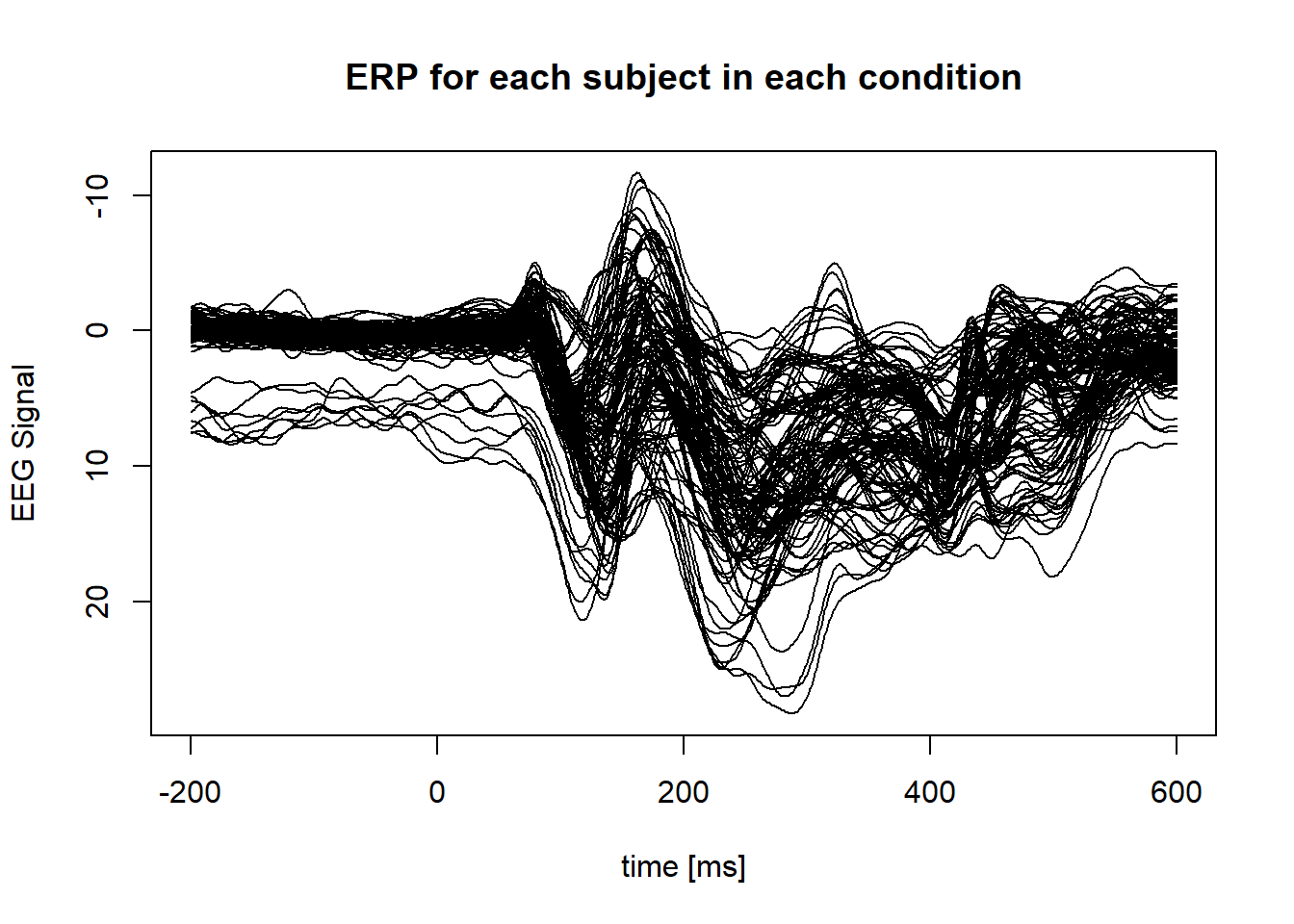
data("attentionshifting_signal")Plot of all the ERP of the O1 electrode :
erp <- t(attentionshifting_signal)
ms <- as.numeric(colnames(attentionshifting_signal))
plot(0, ylim = rev( range( erp)), xlim  = range(ms), type = "n",
     xlab = "time [ms]", ylab = "EEG Signal", main = "ERP for each subject in each condition")
for(i in 1:ncol(erp) ){
  lines(y = erp[,i],x = ms)
}
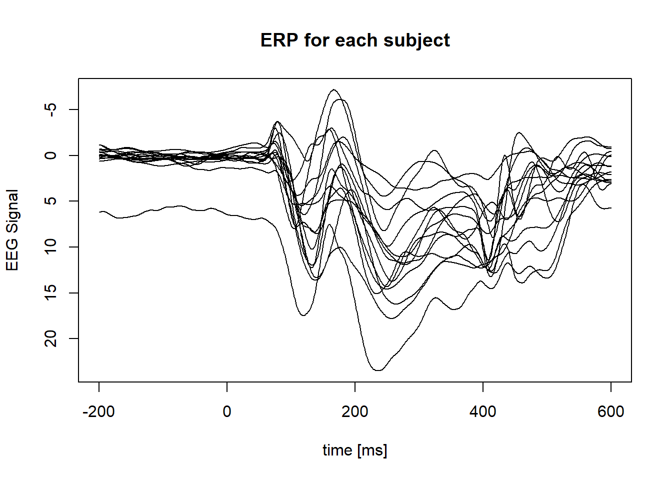
Plot ERP of each subject (average across condition):
erpm <- aggregate(attentionshifting_signal, by = list(
  attentionshifting_design$id), FUN = mean)
erpm <- t(erpm[,-1])
ms <- as.numeric(colnames(attentionshifting_signal))
plot(0, ylim = rev( range( erpm)), xlim  = range(ms), type = "n",
     xlab = "time [ms]", ylab = "EEG Signal", main = "ERP for each subject")
for(i in 1:ncol(erpm) ){
  lines(y = erpm[,i],x = ms)
}
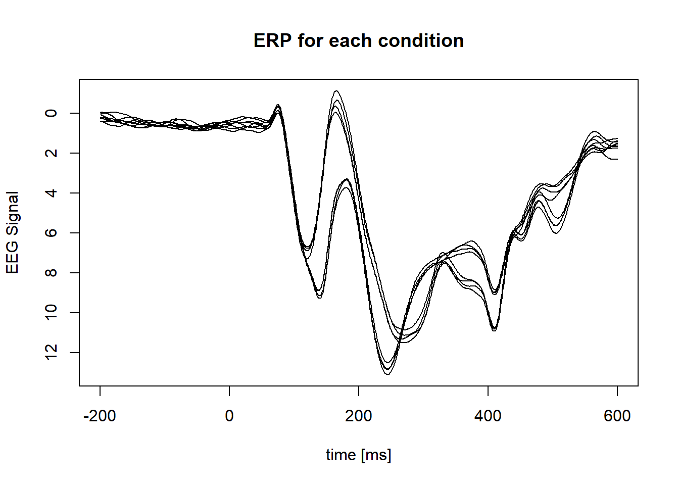
Plot ERP of condition (average across subject):
erpm <- aggregate(attentionshifting_signal, by = list(
  interaction(attentionshifting_design$visibility,
  attentionshifting_design$emotion,attentionshifting_design$direction)), FUN = mean)
erpm <- t(erpm[,-1])
ms <- as.numeric(colnames(attentionshifting_signal))
plot(0, ylim = rev( range( erpm)), xlim  = range(ms), type = "n",
     xlab = "time [ms]", ylab = "EEG Signal", main = "ERP for each condition")
for(i in 1:ncol(erpm) ){
  lines(y = erpm[,i],x = ms)
}
Plot ERP of condition 16ms and 166ms of visibility, average across all other condition, all subjects :
erpm <- aggregate(attentionshifting_signal, by = list(
  attentionshifting_design$visibility), FUN = mean)
condition <- erpm[,1]
erpm <- t(erpm[,-1])
ms <- as.numeric(colnames(attentionshifting_signal))
plot(0, ylim = rev( range( erpm)), xlim  = range(ms), type = "n",
     xlab = "time [ms]", ylab = "EEG Signal", main = "ERP of 16ms and 166ms")
lines(y = erpm[,1],x = ms,lty = 1)
lines(y = erpm[,2],x = ms,lty = 2)
legend("left", legend = condition,lty = c(1,2))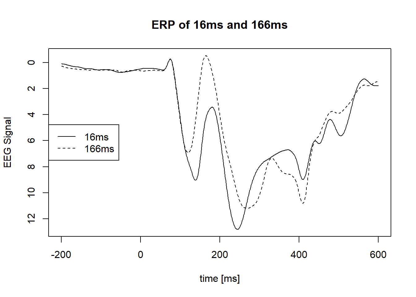
Testing the difference between conditions
In the last plot, we see a difference of brain activity between those two conditions, from 100ms to 250ms. However, we cannot rely on the graphical analysis and we need a statistical test to be able to affirm that this observation is caused by an underlying effect of the visibility instead of just noise.
Several solutions may results to bad statistical decision.
First we could perform around 800 tests (from -200 to 600 ms), at each time and report significant time will results produce a lot of type I error. And even with pure noisy data we will report significant values all the time. With 800 independent tests (which are not) of pure noise data, we have a probability of \(p = 1-(1-0.05)^{800} \approx 1\) to report a significant time-points. This probability is called the family wise error rate (FWER) and we need to control it in order to make a meaningful statistical decision. A second bad approach is select a time-frame based on the plot above, make the average of this time-frame then perform only one test. This approach has the same problems because this procedure will select the most significant results and it will be significant with high probability even under pure noise. However in order perform a meaningful test, we want to use a procedure that control the FWER and the typical Bonferroni or Holm corrections are not powerful enough. The Bonferroni correction will divide the individual \(\alpha\) thresholds by the number of tests and with 800 tests, we will miss a lot of true effects.
The permuco package is designed to compute cluster-mass statistics (Maris and Oostenveld 2007) which control the FWER and has a high power if the effect are highly correlated. It is the case for EEG data which shows high temporal correlated : if an effect appears at time \(t\), it has a high probability to appears at time \(t+1\) and \(t-1\). This allow us to interpret effects into cluster of adjacent time frames. We define all adjacent times which statistics are above a threshold as a cluster and then compute the cluster-mass by taking the sum of those statistics. To compute the p-value of a cluster, we compute the cluster-mass distribution by permutation (Kherad Pajouh and Renaud 2010, @winkler_permutation_2014, @kherad–pajouh_general_2015) and by comparing this distribution to the observed cluster-mass we deduce a p-value.
We use the permuco package to perform this test on our data. First, we delete the time frame below zero; there cannot be an effect of the images before showing them. And then we use the clusterlm function. Note that the formula use their term “Error()” which is similar the aov() function. In both case it is used for repeated measures ANOVA to specify the “within” factors.
ms <- as.numeric(colnames(attentionshifting_signal))
clustermass <- clusterlm(attentionshifting_signal[, ms>=0] ~ visibility*emotion*direction
    + Error(id/(visibility*emotion*direction)), data = attentionshifting_design)
This function will take several minutes to run. It will perform the 7 tests, around 600ms and 5000 permutations. You can see the results quickly using the plot function.
plot(clustermass)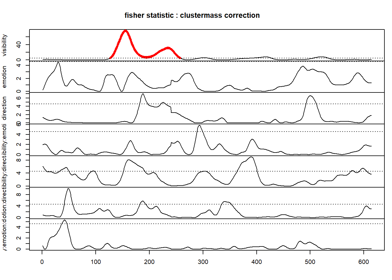
It displays the 7, tests and in red the significant time-points. There is a significant cluster for the effect of visibility between 120ms and 150ms. The dashed lines represent the threshold and is set by default to the \(95\) percentile of the parametric statistics. We print the results to have more information on the effects.
clustermass## Effect: visibility.
## Statistic: ().
## Permutation Method: .
## Number of Dependant Variables: .
## Number of Permutations: .
## Multiple Comparisons Procedure: clustermass.
## Threshold: 4.60011.
## Mass Function: .
## Table of clusters.
##
## start end cluster mass P(>mass)
## 1 127 257 3559.14974 0.0012
## 2 294 309 85.01965 0.3774
## 3 391 427 234.87791 0.2062
## 4 506 533 191.57618 0.2476
##
##
## Effect: emotion.
## Statistic: ().
## Permutation Method: .
## Number of Dependant Variables: .
## Number of Permutations: .
## Multiple Comparisons Procedure: clustermass.
## Threshold: 4.60011.
## Mass Function: .
## Table of clusters.
##
## No cluster above the threshold.
##
##
## Effect: direction.
## Statistic: ().
## Permutation Method: .
## Number of Dependant Variables: .
## Number of Permutations: .
## Multiple Comparisons Procedure: clustermass.
## Threshold: 4.60011.
## Mass Function: .
## Table of clusters.
##
## start end cluster mass P(>mass)
## 1 182 196 89.29120 0.3484
## 2 222 230 43.15493 0.4152
## 3 492 511 117.22493 0.3086
##
##
## Effect: visibility:emotion.
## Statistic: ().
## Permutation Method: .
## Number of Dependant Variables: .
## Number of Permutations: .
## Multiple Comparisons Procedure: clustermass.
## Threshold: 4.60011.
## Mass Function: .
## Table of clusters.
##
## start end cluster mass P(>mass)
## 1 289 299 58.91771 0.3924
##
##
## Effect: visibility:direction.
## Statistic: ().
## Permutation Method: .
## Number of Dependant Variables: .
## Number of Permutations: .
## Multiple Comparisons Procedure: clustermass.
## Threshold: 4.60011.
## Mass Function: .
## Table of clusters.
##
## start end cluster mass P(>mass)
## 1 1 8 42.56374 0.4208
## 2 33 49 89.59733 0.3530
## 3 94 97 18.61131 0.4532
## 4 152 191 268.04807 0.1804
## 5 364 401 279.00621 0.1758
## 6 577 581 23.57752 0.4472
## 7 592 604 67.14642 0.3880
##
##
## Effect: emotion:direction.
## Statistic: ().
## Permutation Method: .
## Number of Dependant Variables: .
## Number of Permutations: .
## Multiple Comparisons Procedure: clustermass.
## Threshold: 4.60011.
## Mass Function: .
## Table of clusters.
##
## start end cluster mass P(>mass)
## 1 42 57 127.82364 0.2942
## 2 183 193 58.70748 0.3960
## 3 335 353 100.14845 0.3324
##
##
## Effect: visibility:emotion:direction.
## Statistic: ().
## Permutation Method: .
## Number of Dependant Variables: .
## Number of Permutations: .
## Multiple Comparisons Procedure: clustermass.
## Threshold: 4.60011.
## Mass Function: .
## Table of clusters.
##
## start end cluster mass P(>mass)
## 1 37 46 50.4056 0.4226The cluster shows in the plot has a cluster-mass of 3559.15 with a p-value of 0.0012. The cluster-mass distribution can be plotted for this effect using :
mass_distr = clustermass$multiple_comparison$visibility$clustermass$distribution
plot(density(mass_distr), main = "clustermass null distributin of visibility",
     xlab="",ylab="")
abline(v=mass_distr[1])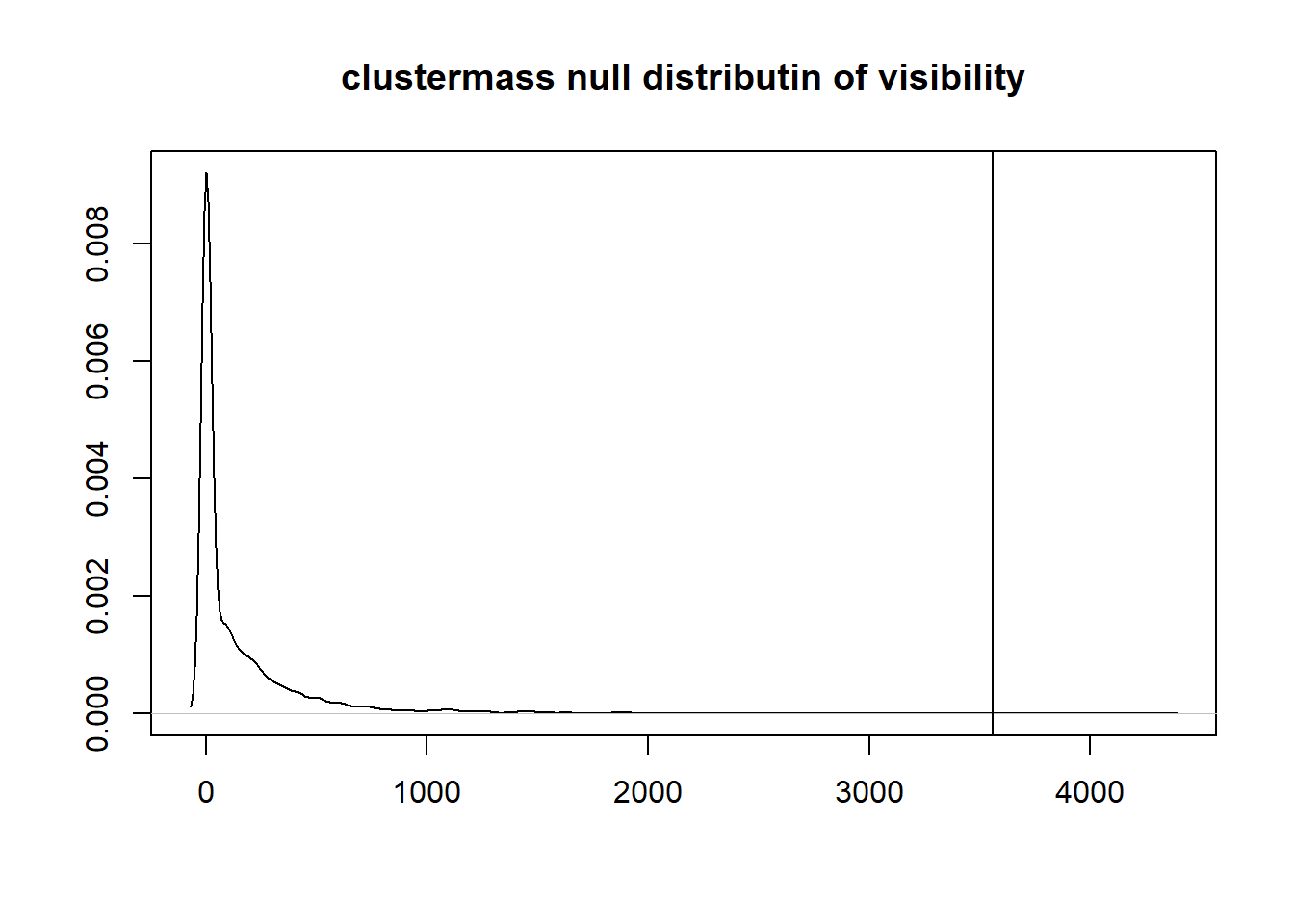
Bibliography
Kherad Pajouh, Sara, and Olivier Renaud. 2010. “An Exact Permutation Method for Testing Any Effect in Balanced and Unbalanced Fixed Effect ANOVA.” Computational Statistics & Data Analysis 54: 1881–93. https://doi.org/10.1016/j.csda.2010.02.015.
Kherad-Pajouh, Sara, and Olivier Renaud. 2015. “A General Permutation Approach for Analyzing Repeated Measures ANOVA and Mixed-Model Designs.” Statistical Papers 56 (4): 947–67. https://doi.org/10.1007/s00362-014-0617-3.
Maris, Eric, and Robert Oostenveld. 2007. “Nonparametric Statistical Testing of EEG- and MEG-Data.” Journal of Neuroscience Methods 164 (1): 177–90. https://doi.org/10.1016/j.jneumeth.2007.03.024.
Winkler, Anderson M., Gerard R. Ridgway, Matthew A. Webster, Stephen M. Smith, and Thomas E. Nichols. 2014. “Permutation Inference for the General Linear Model.” NeuroImage 92: 381–97. https://doi.org/10.1016/j.neuroimage.2014.01.060.